HCX Perftest Issue

Introduction

VMware HCX is a great tool, which simplifies VM migrations between on-prem to on-prem or on-prem to cloud at scale. I’ve worked with many different VM migration tools before and what I particularly like about HCX is it’s ability to stretch network subnets between source and destination environments. It reduces (or completely removes) the need to re-IP VMs, which simplifies the migration and reduces the risk of inadvertently introducing issues into migrated applications.

Perftest Tool

HCX is a complex set of technologies and getting initial deployment right is key to building a reliable migration fabric. Perftest is a CLI tool available on interconnect (IX) and network extension (NE) HCX appliances, which allows you to perform validation testing to ensure everything is functioning correctly, as well as provide you a performance baseline. To run this tool you will need to SSH into HCX Manager, enter CCLI and then go to one of your IX or NE appliances:

# ccli
# list
# go 0
# perftest all

Issue Description

There is one issue you can come across, when running perftest, where it partially completes with the following errors:

Message Error: map[string]interface {}{“grpc_code”:14, “http_code”:503, “http_status”:”Service Unavailable”, “message”:”rpc error: code = Unavailable desc = transport is closing”}

and

Internal failure happens. Err: http.Post(https://appliance_ip:9443/perftest/stoptest) return statusCode: 503

Solution

The reason for this error is blocked connectivity on port TCP/4500. HCX uses ports UDP/4500 and UDP/500 for establishing tunnels between IX and NE appliance pairs, but that’s not enough for perftest.

In the very beginning of the perftest it gives you a hint, but it’s easy to overlook. This requirement is not well documented (at least at the time of writing), so keep that in mind next time you deploy HCX.

RecoverPoint VE: iSCSI Network Design

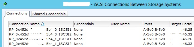
RecoverPoint is a great storage replication product, which supports Continuous Data Protection (CDP) and gives you RPO figures measured in second compared to a standard asynchronous storage-based replication solutions, where RPO is measured in minutes or even hours.

RecoverPoint comes in three flavours:

• RecoverPoint SE/EX/CL – physical appliance for replication between VNX (RecoverPoint/SE), VNX/VMAX/VPLEX (RecoverPoint/EX) or EMC and non-EMC (RecoverPoint CL) storage arrays.
• RecoverPoint VE – virtual edition of RecoverPoint which is installed as a VM and supports the same SE/EX/CL versions.
• RecoverPoint for Virtual Machines – also a virtual appliance but is array-agnostic and works at a hypervisor level by replicating VMs instead of LUNs.

In this blog post we will be discussing connectivity options for RecoverPoint VE (SE edition). Make sure to not confuse RecoverPoint VE and RecoverPoint for Virtual Machines as it’s two completely different products.

VNX MirrorView ports

MirrorView is an another EMC replication solution integrated into VNX arrays. If there’s a MirrorView enabler installed, it will claim itself the first FC port and the first iSCSI port. When patching VNX iSCSI ports make sure to NOT use the ports claimed by MirrorView.

If you use 1GbE (4-port) I/O modules you can use three ports per SP (all except port 0) and if you have 10GbE (2-port) I/O modules you can use one port per SP. I will talk about workarounds for this in the next blog post.

RPA appliance iSCSI vNICs

Each RecoverPoint appliance has two iSCSI NICs, which can be configured on either one or two subnets. If you use one 10Gb port on each SP as in the example above, then you’re forced to use one subnet. Because you obviously need at least two ports on each SP to have two networks.

If you have 1Gb modules in your VNX array, then you will most likely have two 1Gb iSCSI ports connected on each SP. In that case you can use two iSCSI subnets to reduce the number of iSCSI sessions between RPAs and a VNX.

On the vSphere side you will need to create one or two iSCSI port groups, depending on how many subnets you’ve decided to allocate and connect RPA vNICs accordingly.

VNX iSCSI Connections

RecoverPoint clusters are deployed and connected using a special tool called Deployment Manager. It assigns all IP addresses, connects RecoverPoint clusters to VNX arrays and joins sites together.

Once deployment is finished you will have iSCSI connections created on the VNX array. Depending on how many iSCSI subnets you’re using, iSCSI connections will be configured accordingly.

1. One Subnet Example

Lets look at the one subnet topology first. In this example you have one 10Gb port per VNX SP and two ports on each of the two RPAs all on one subnet. When you right click on the storage array in Unisphere and select iSCSI > Connections Between Storage Systems you should see something similar to this.

As you can see ports iSCSI1 and iSCSI2 on RPA0 and RPA1 are mapped to two ports on the storage array A-5 and B-5. Four RPA ports are connected to two VNX ports which gives you eight iSCSI initiator records on the VNX.

2. Two Subnets Example

If you connect two 1Gb ports per VNX SP and decide to use two subnets, then each SP will have one port on each of the two subnets. Same goes for the RPAs. Each RPA will have one vNIC connected to each subnet.

iSCSI connections will be set up a little bit differently now. Because only the VNX and RPA ports which are on the same subnet should be able to talk to each other.

Every RPA in this example has one IP on the xxx.xxx.46.0/255.255.255.192 subnet (iSCSI A) and one IP on the xxx.xxx.46.64/255.255.255.192 subnet (iSCSI B). Similarly, ports A-10 and B-10 on the VNX are configured on iSCSI A subnet. And ports A-11 and B-11 are configured on iSCSI B subnet. Because of that, iSCSI1 ports are mapped to ports A-10/B-10 and iSCSI2 ports are mapped to ports A-11/B-11.

As we are using two subnets in this example instead of 4 RPA ports by 4 VNX ports = 16 iSCSI connections, we will have 2 RPA ports by 2 VNX ports (subnet iSCSI A) + 2 RPA ports by 2 VNX ports (subnet iSCSI B) = 8 iSCSI connections.

Conclusion

The goal of this post was to discuss the points which are not very well explained in RecoverPoint documentation. It’s not a comprehensive guide by any means. You can find the full deployment procedure with prerequisites, installation and configuration steps in EMC RecoverPoint Installation and Deployment Guide.

Traffic Load Balancing in Cisco UCS

Whenever I deploy a Cisco UCS at a customer the question I get asked a lot is how traffic flows within the system between VMs running on the blades and FEX modules, FEX modules and Fabric Interconnects and finally how it’s uplinked to the network core.

Cisco has a range of CNA cards for UCS blades. With VIC 1280 you get 8 x 10Gb ports split between two FEX modules for redundancy. And FEX modules on their own can have up to 8 x 10Gb Fabric Interconnect facing interfaces, which can give you up to 160Gb of bandwidth per chassis. And all these numbers may sound impressive, but unless you understand how your VMs traffic flows through UCS it’s easy to make wrong assumptions on what per VM and aggregate bandwidth you can achieve. So let’s dive deep into UCS and shed some light on how VM traffic is load-balanced within the system.

UCS Hardware Components

Each Fabric Extender (FEX) has external and internal ports. External FEX ports are patched to FIs and internal ports are internally wired to the blade adapters. FEX 2204 has 4 external and 16 internal and FEX 2208 has 8 external and 32 internal ports.

External ports are connected to FIs in powers of two: 1, 2, 4 or 8 ports per FEX and form a port channel (make sure to use “Port Channel” link grouping preference under Chassis/FEX Discovery Policy). Same rule is applied to blade Virtual Interface Cards (VIC). The most common VIC 1240 and 1280 have 4 x 10Gb and 8 x 10Gb ports respectively and also form a port channel to the internal FEX ports. Every VIC adaptor is connected to both FEX modules for redundancy.

Fabric Interconnects are then patched to your network core and FC Fabric (if you have one). Whether Ethernet uplinks will be individual uplinks or port channels will depend on your network topology. For fibre uplinks the rule of thumb is to patch FI A to your FC Fabric A and FI B to FC Fabric B, which follows the common FC traffic isolation principle.

Virtual Circuits

To provide network and storage connectivity to blades you create virtual NICs and virtual HBAs on each blade. Since internally UCS uses FCoE to transfer FC frames, both vNICs and vHBAs use the same 10GbE uplinks to send and receive traffic. Worth mentioning that Cisco uses Data Center Bridging (DCB) protocol with it’s sub-protocols Priority Flow Control (PFC) and Enhanced Transmission Selection (ETS), which guarantee that FC frames have higher priority in the queue and are processed first to ensure low latency. But I digress.

UCS assigns a virtual circuit to each virtual adaptor, which is a representation of how the traffic traverses the system all the way from the VIC port to a FEX internal port, then FEX external port, FI server port and finally a FI uplink. You can trace the full path of each virtual adaptor in UCS Manager by selecting a Service Profile and viewing the VIF Paths tab.

In this example we have a blade with four vNICs and two vHBAs which are split between two fabrics. All virtual adaptors on fabric A are connected through VIC port channel PC-1283 which is represented as port channel PC-1025 on the FEX A side. Then traffic leaves FEX A and reaches the Fabric Interconnect A which sends the traffic out to the network core through port channel A/PC-1.

You can also get the list of port channels from the FI CLI:

# connect nxos
# show port-channel summary

Network Load Balancing

Now that we know how all components are interconnected to each other, let’s discuss the traffic flow in a typical VMware environment and how we achieve the massive network throughput that UCS provides.

As an example let’s take a look at the vSwitch where your VM Network port group is configured. vSwitch will have two uplinks – one goes to Fabric A and the other one to Fabric B for redundancy. Default load balancing policy on a vSwitch is “Route based on the originating port ID”, which essentially pins all traffic for a VM to a particular uplink. vSphere makes sure that VMs are evenly distributed between the uplinks to use all network bandwidth available.

From each uplink (or vNIC in UCS world) traffic is forwarded through an adapter port channel to a FEX, then to a Fabric Interconnect and leaves UCS from a FI uplink. Within UCS traffic is distributed between port channel members using source/destination IP hash algorithm. Which is even more granular and is capable of very efficient traffic distribution between all members of a port channel all the way up to your network core.

If you look at the vSwitch you’ll see that with UCS each uplink shows the maximum available bandwidth from vNIC and is not limited to a port channel member speed of 10Gb. Why is this so powerful? Because with UCS you don’t need to slice adapter’s available bandwidth between different types of traffic. Even though you provision multiple vNICs and vHBAs for the vSphere hosts, UCS uses the same port channel links (20Gb in the example below) from the VIC adapter to transfer all traffic and takes care of load balancing for you.

You may legitimately ask, if UCS uses the same pipe to transfer all data regardless of which vSwitch uplink is being used, then how can I make sure that different types of traffic, such as vMotion, storage, VM traffic, replication, etc, do not compete for the same pipe? First you need to ask yourself if you can saturate that much bandwidth with your workloads. If the answer is yes, then you can use another great feature available in UCS, which is QoS. QoS lets you assign a minimum available bandwidth guarantee on a per vNIC/vHBA basis. But that’s a topic for another blog post.

References

In this post I tried to summarise the logic behind UCS traffic distribution. If you want to dig deeper in UCS network architecture, then there’re a lot of great bloggers out there. I would like to call out the following authors:

• Brad Hedlund – if you want to better understand overall UCS architecture and network best practices, Bred has a great series of videos:
  • Cisco UCS Networking videos (in HD), Updated & Improved!
• Colin Lynch (UCSguru) – this blog is dedicated specifically to UCS. If you want to know more about the virtual circuits, I would recommend these two blog posts:
  • Understanding UCS VIF Paths
  • Under the Cisco UCS Kimono
• Matthew Oswalt – Keeping It Classless is a blog which is geared more towards DevOps, but also has a few UCS articles, I found this one particularly useful:
  • Cisco UCS Port-Channeling

 

Force10 MXL Switch: Port Numbering

This is a quick cheat sheet fro MXL port numbering schema, which might seem a bit confusing if you see a MXL switch for the first time.

Above is the picture of the switches that I’ve worked with. On the right we have a 2-Port 40GbE built-in module. And then there’re two expansion slots – slot 0 in the middle and slot 1 on the left. Each module has 8 ports allocated to it. The reason being that you can have 2-Port 40-GbE QSFP+ modules in each of the slots, which can operate in 8x10GbE mode. You will need QSFP+ to 4xSFP+ breakout cables, but that’s not the most common scenario anyway.

As we have 8 ports per slot, it would look something like this:

This picture is more for switch stacking, but the rightmost section should give you a basic idea. One of the typical MXL configurations is when you have a built-in 40GbE module for stacking and one or two 4-Port SFP+ expansion modules in slots 0 and 1. In that case your port numbers will be: 33 and 37 for 40GbE ports, 41 to 44 in expansion slot 0 and 49 to 52 in expansion slot 1.

As you can see for QSFP+ module switch breaks 8 ports in two sets of 4 ports and picks the first number in each set for 40GbE ports. And for SFP+ modules it uses consecutive numbers within each slot and then has a 4 port gap.

Port numbering is described in more detail in MXL’s switch configuration guide, which you can use for your reference. But this short note might help someone to quickly knock that off instead of browsing through a 1000 page document.

Also, I’ve seen pictures of MXL switches with a slightly different port numbering: 41 to 48 in slot 0 and 33 to 40 in slot 1. Which seems like a mirrored version of the switch with a built-in module on the opposite side of it. I’m not sure if it’s just an older version of the same switch, but keep in mind that you might actually have the other variation of the MXL in your blade chassis.

Switching Logic

If you are a junior admin in a small to medium organization then building campus network is simple. Buy several switches, connect desktops and switches together and that’s it. You don’t need any additional configuration, all switches work right out of the box. However, it’s important to understand how packet switching work to troubleshoot problems that can show up later in your work.

Switching works on TCP/IP Layer 2. It means that networking hardware logic operates with MAC addresses. Each time switch receives a packet from any workstation or server it remembers its MAC address and port it was received from. It’s called MAC address or switching table. When somebody wants to send a packet to an other host with particular IP address he sends an ARP request packet. Like tell me who has 12.34.56.78 IP address. Host replies with its MAC address and sender can form a package to it.

Initially switch has empty switching table and does not know where to send packets. When switch doesn’t have particular MAC address in its table it forwards (floods) the packet to all ports. If the next switch doesn’t know this MAC, it further forwards the packet. When packet finally reaches its destination, host answers and switch adds its MAC address into the table.

If you don’t use VLANs, all switches in your network form a broadcast domain. It means that when host sends a broadcast message, ARP request for example, and host with this IP address is powered off then this ARP request will traverse the whole network. It’s important to bear in mind that if you have many hosts in your network, broadcast messages can eventually slow it down. VLANs are usually a solution here.

Permanently map network drive in Windows

Have you ever run into an issue when after mapping a network drive and saving login/password you end up with disconnected drive after a reboot? To overcome this problem use command line with the following switches to net use routine:

net use w: \\server\share /savecred /persistent:yes

Then enter your username and password and that seems to be it.

But I had a problem when network drive doesn’t map with error: “Invalid username/password”. Even though they are correct. If you run into a similar problem include username and password into the command like this:

net use w: \\server\share password /savecred /persistent:yes /user:username

Present NetApp iSCSI LUN to Linux host

Consider the following scenario (which is in fact a real case). You have a High Performance Computing (HPC) cluster where users usually generate hellova research data. Local hard drives on a frontend node are almost always insufficient. There are two options. First is presenting a NFS share both to frontend and all compute nodes. Since usually compute nodes  connect only to private network for communication with the frontend and don’t have public ip addresses it means a lot of reconfiguration. Not to mention possible security implications.

The simpler solution here is to use iSCSI.  Unlike NFS, which requires direct communication, with iSCSI you can mount a LUN to the frontend and then compute nodes will work with it as ordinary NFS share through the private network. This implies configuration of iSCSI LUN on a NetApp filer and bringing up iSCSI initiator in Linux.

iSCSI configuration consists of several steps. First of all you need to create FlexVol volume where you LUN will reside and then create a LUN inside of it. Second step is creation of initiator group which will enable connectivity between NetApp and a particular host.  And as a last step you will need to map the LUN to the initiator group. It will let the Linux host to see this LUN. In case you disabled iSCSI, don’t forget to enable it on a required interface.

vol create scratch aggrname 1024g
lun create -s 1024g -t linux /vol/scratch/lun0
igroup create -i -t linux hpc
igroup add hpc linux_host_iqn
lun map /vol/scratch/lun0 hpc
iscsi interface enable if_name

Linux host configuration is simple. Install iscsi-initiator-utils packet and add it to init on startup. iSCSI IQN which OS uses for connection to iSCSI targets is read from /etc/iscsi/initiatorname.iscsi upon startup. After iSCSI initiator is up and running you need to initiate discovery process, and if everything goes fine you will see a new hard drive in the system (I had to reboot). Then you just create a partition, make a file system and mount it.

iscsiadm -m discovery -t sendtargets -p nas_ip
fdisk /dev/sdc
mke2fs -j /dev/sdc1
mount /dev/sdc1 /state/partition1/home

I use it for the home directories in ROCKS cluster suite. ROCKS automatically export /home through NFS to compute nodes, which in their turn mount it via autofs. If you intend to use this volume for other purposes, then you will need to configure you custom NFS export.

VMware Tools update issue

Recently I decided to update VMware Tools on VMs because most of them showed Out of date in VI client. For some reason several Linux VMs didn’t update even though VI client showed no error. I tried to update from inside VM by running /usr/sbin/vmware-tools-upgrade and it showed that there is not enough space in /tmp. I enlarged /tmp from 128 to 512MB and update went fine this time.

Take into account that:

1. Windows VM will most likely be rebooted after update.
2. In Linux VMmware Tools may not start automatically. If it’s the case start it manually by calling /etc/init.d/vmware-tools start.
3. Network interfaces in Linux may go down after VMware Tools update. Boot them manually.

 

Solaris NIC settings

Today I faced a problem with network configuration on an ancient Solaris 7 RISC. Symptoms: output network speed 2.5MB/s, input speed 100KB/s.

netstat -in (-i for interfaces, -n for numbers) showed lots of Ierrs. The reason for that was mismatch in advertised capabilities even though effectively it was 100 FDX at each end. I had following parameters set in /etc/system left from previous admin:

set hme:hme_adv_autoneg_cap=0
set hme:hme_adv_100fdx_cap=1
set hme:hme_adv_100hdx_cap=0
set hme:hme_adv_10hdx_cap=0
set hme:hme_adv_10fdx_cap=0

And for switch it was:

# ndd -get /dev/hme lp_autoneg_cap
1

# ndd -get /dev/hme lp_100fdx_cap
1

# ndd -get /dev/hme lp_100hdx_cap
1

# ndd -get /dev/hme lp_10hdx_cap
1

# ndd -get /dev/hme lp_10fdx_cap
1

So the lesson is: always keep network settings equal on both ends even if they don’t contradict with each other at first sight.